Eshelby established the basis of the micromechanics theory for isotropic body[1]. Afterward it has been extended for anisotropic cases by other researchers, and has become more sophisticated theory; for example, one can see more systematized theory in Mura’s book[2]. In this section, we introduce Eshelby’s ellipsoidal inclusion theory.
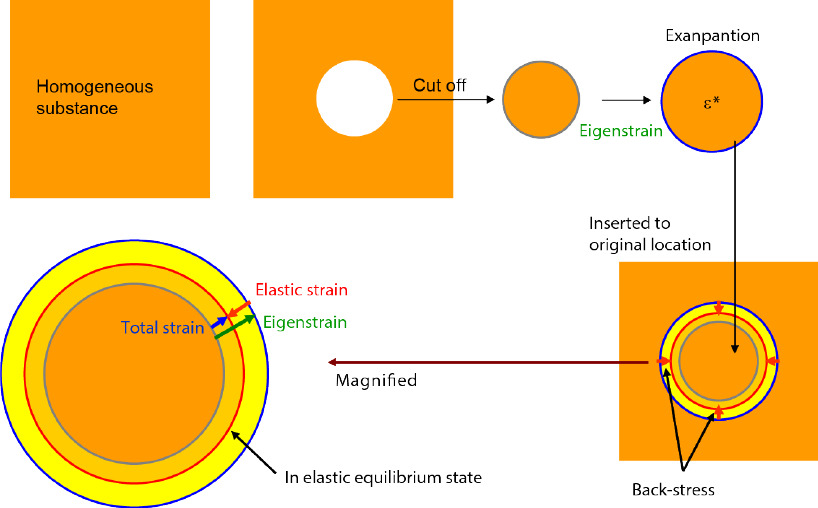
Suppose that only a small part Ω in an originally uniform substance is expanded because of thermal dilatation or a certain transformation. Then, the substance becomes in an internal-stress state. If the surroundings of Ω does not exist, the displacement due to such an intrinsic dilatation of Ω will be larger; the strain expressed by this displacement is not elastic but plastic, which is called eigenstrain or stress-free transformation strain, which is denoted as ϵkl*. However, the surroundings prohibits such an intrinsic dilatation; Ω is shrinked elastically because of the constraint by the surroundings. This elastic strain is denoted as ϵkl. When the total displacement measured referring to the initial state is denoted as u = (u1,u2,u3), the total strain can be written as γkl = ∂uk∕∂xl, which is given by sum of the eigenstrain and elastic strain;
where ϵkl*≠0 in Ω, and ϵ kl* = 0 in the exterior matrix D-Ω. This situation is illustrated in Fig. 1.
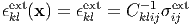
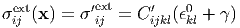
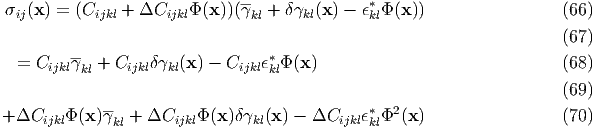
Next suppose that a number of inclusions with an eigenstrain ϵkl* exist in a substance; the spatial distribution of ϵkl* is denoted as ϵ kl*(x). When x is located inside Ω (i.e., x ∈ Ω), ϵkl*(x) = ϵ kl*, and when x is outside Ω (i.e., x ∋ Ω), ϵ kl*(x) = 0. In the case where the elastic constants Cijkl of matrix are equal to those of inclusions, Hooke’s law can be written as
which holds at each position x.
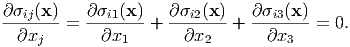
When the total displacement u or total strain γ are known, all the stress/strain fields can be analyzed. To do this, we have to solve the following elastic-equilibrium equation:
| (3) |
Hereafter, the summation convention is applied when the same subscripts appear. Substituting Eq. (70) into Eq. (3), we obtain
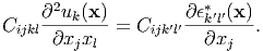
| (4) |
To solve this equation, we transform uk(x) and ϵk′l′*(x) into the Fourier
forms: ũk(g) and  k′l′*(g). Then, in the Fourier spcace, Eq. (4) is written as

| (5) |
The solution of Eq. (5) is given by

| (6) |
where Kik ≡ Cijklgjgl and the subscripts k′l′ are changed to mn. When g is denoted as gg (g is the unit vector, and g is the magnitude of the vector),

| (7) |
Hence, Eq. (6) is written as

| (8) |
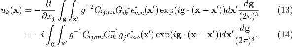
and hence the expression of ∂uk∕∂xl in the Fourier space is

| (9) |
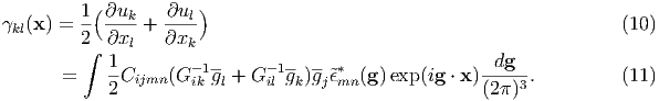
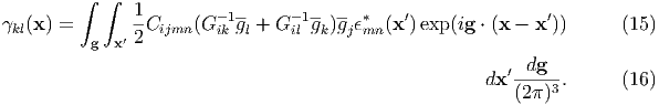
where {A(x)}g means the Fourier transform of A(x). Therefore, the symmetric total strain γkl(x) is expressed as
Moreover, since
| (12) |
from Eq. (8)
and from Eq. (11) Equations (11), (14) and (16) are the general solutions of the elastic-equilibrium equation (3) for an elastically homogeneous substance.
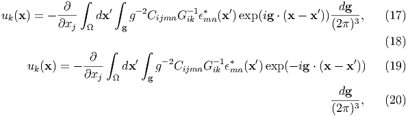
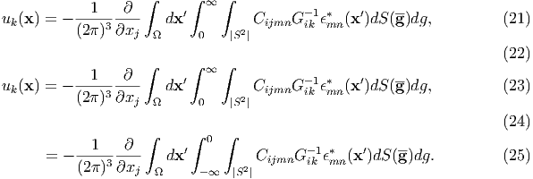
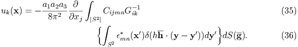
Hereafter, we consider the case wehre there is one inclusion Ω that has the eigenstrain ϵ*(x′). Since ϵ*(x′) = 0 for x′∋ Ω, Eq. (14) is
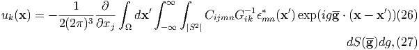
because g-2C ijmnGik-1ϵ mn*(x′) is an even function of g, and the integral range g-space is invariable when dg →-dg. By using the relation of dg = dg1dg2dg3 = dS(g)dg = g2dS(g)dg, Eq. (20) is expressed as From the upper and lower equations in Eq. (25), we obtain where the integral ∫ |S2|dS(g) is performed on the surface of the unit sphere S2, with g the vector variable moving on the surface |S2|. By using the characteristics with regard to the delta function
| (28) |
we obtain
Since the delta function has a following characteristics
| (30) |
we have to seek x′ in Ω so as to satisfy g ⋅ (x - x′) = 0.
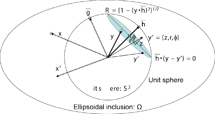
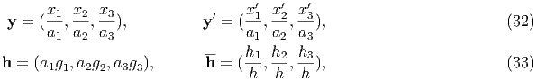
We first deal with the integral ∫ Ωϵmn*(x′)δ(g ⋅ (x - x′))dx′ in Eq. (29), where we ragard that x and g are fixed, and consider the case where x = (x1,x2,x3) is located in the ellipsoidal inclusion Ω with radii a1, a2, and a3:
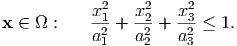
| (31) |
Transformations of variables are made as follows:
where |h| = 1 and h = |h| = 1∕2. When the vector variable
x′ moves inside the ellipsoidal inclusion Ω, y′ moves inside the unit sphere S2 (see Fig.
2):
1∕2. When the vector variable
x′ moves inside the ellipsoidal inclusion Ω, y′ moves inside the unit sphere S2 (see Fig.
2):

| (34) |
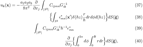
Since dx = a1a2a3dy and g ⋅ (x - x′) = hh ⋅ (y - y′), Eq. (29) is written as
Here, y′ is expressed using the cylindrical coordinate (z,r,ϕ); the origin O of the coordinate is the cross point of the vector h and the plane that is normal to h and is passing on the point y, as shown in Fig. 2. Then, the following relations hold:

In Eq. (36), ∫ S2ϵmn*(x′)δ(hh ⋅ (y - y′))dy′ is performed under the fixed y and h. Therefore,
where the latter formula is obtained under the condition that the eigenstrain is uniform in Ω (i.e., ϵmn*(x′) = ϵ mn*). By using the following geometric relation, R2 = 1 - (y ⋅h)2 = 1 - (x ⋅g)2∕h2 (see Fig. 2), we obtain Substituting Eq. (41) into Eq. (40), we obtain After all, we can express the symmetric total strain as It is noted that the total strain in Ω is uniform, being independent of x.When x is located in the exterior matrix (i.e., x ∋ Ω), it is quite complicated to calculate the outside fields because the hatched area displayed in Fig. 2, which satisfies h ⋅ (y - y′) = 0, does not exist for any y′ when y ⋅h > 1. Taking into account this matter, Cheng and Mura has derived the outside field of ellipsoidal inclusion[3].
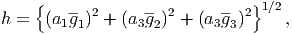
As found from Eq. (43), the total strain γik in the inclusion Ω can be written in the following form:

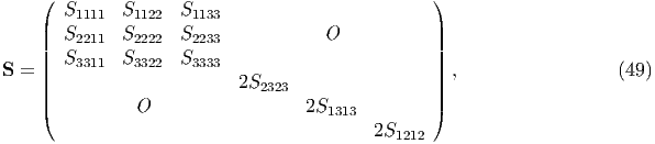
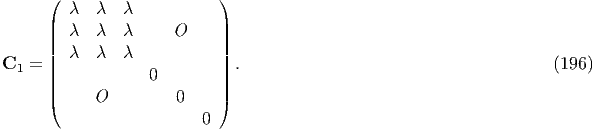
General ellipsoidal shape As seen in Eq. (43), the most general form of the fourth-rank Eshelby tensors for the arbitrary shape of ellipsoidal inclusion are given by
where the surface integral is performed over the unit sphere |S2| that is made by unit vector g, Cjlmn denotes the elastic constants of matrix, gp is a component of g, and (a1, a2, a3) denote the radii of the ellipsoidal inclusion.
Cylindrical shape For cylindrical (needle) shape, i.e., a3∕a1(= a3∕a2) →∞, S tensors reduce to
where the line integral is performed over the unit circle SL normal to the x 3 (i.e., a3) direction.Plate-disc shape For the plate-disc inclusion with zero aspect ratio i.e., a3∕a1(= a3∕a2) → 0, S tesors further reduce to
where the vector g is taken to be normal to the disc basal plane.In general, the principle axes of ellipsoidal inclusion are not always consistent with the crystallographic axes (in which the elastic constants, strain and stress etc are defined). In such a case, it is convenient to transform the elastic constants of crystal-coordinate system into those of the inclusion-coordinate system:

Moreover, there are often cases that we want to use the Eshelby tensors of 6 × 6 matrix form, because the elastic-constant tensors can be reduced to 6 × 6 matrix form, and the tensor calculation becomes more simple. As found from Eqs. (45)-(46), there is a following symmetry Sijkl = Sjikl = Sijlk and Sijkl≠Sklij. Therefore, the Eshelby-tensor matrix S can be expressed as
When the elastic constants of inclusion are different from those of matrix, we have to reconsider the elastic-equilibirum equation (this will be discussed in the later section). Here, a convenient method that does not require the reconsideration of the elastic-equilibirum equation is presented. If the elastic constants of inclusion can be somehow regarded as the same as those of matrix by modifying the eigenstrain, we can deal with the same elastic-equilibrium equation as well as in the previous sections. There is a well-known method, so-called equivalent inclusion method, to solve the elastic inhomogeneity problem.
Type-I equivalent inclusion When an ellipsoidal inclusion has no eigenstrain but elastic constants C′ijkl different from those of matrix Cijkl, stress and strains due to an applied external stress becomes not uniform because of the elastic inhomogeneity; the stress and strain disturbances, which are denoted as σ′ij and γkl, are tried to be reproduced using an equivalent inclusion.
When there is no inclusion, a uniform strain ϵkl0 is caused by external stress:

We have to seek the equivalent eigenstrain ϵkl* so as to satisfy Eq. (51). Note that if the elastic constants are the same, the stress and strain associated with the external stress are uniform, even when the inclusion has an eigenstrain. Furthermore, the intrinsic (original) eigenstrain ϵ′kl* of the inclusion does not appear in Eq. (51). This is because the initial internal-stress state due to ϵ′kl* in the absence of external stress is regarded as a standard. These matters are related with Colonnetti’s theorem, which is described in Sec. 3.
Type-II equivalent inclusion We consider the case where an ellipsoidal inclusion has both eigenstrain ϵ′kl* and different elastic constants C′ijkl. The internal stress due to the inhomogeneous inclusion is tried to be reproduced using an equivalent inclusion.
The stress inside the inclusion is expressed as
We have to seek the equivalent eigenstrain ϵkl** so as to satisfy Eq. (52).
In the previous section, we derived Eqs. (11), (16) and (14) as solutions of linear elastic-equilibrium equation (3) for elastic homogeneity, and obtained Eq. (43) for the special case where there is one ellipsoidal inclusion in the substance. However, the following two points has not been discussed yet.
 mn*(g) exp(ig ⋅ x),
shows a singularity at g = 0, because Gik = Cipkqgpgq has no inverse
matrix. In the derivation of Eq. (43) for ellipsoidal inclusion, we have avoid
calculating the integrand at g = 0, by utilizing the characteristics of delta
function δ(x). If we treat Eq. (11) more generally, how should we deal with
this singularity?
mn*(g) exp(ig ⋅ x),
shows a singularity at g = 0, because Gik = Cipkqgpgq has no inverse
matrix. In the derivation of Eq. (43) for ellipsoidal inclusion, we have avoid
calculating the integrand at g = 0, by utilizing the characteristics of delta
function δ(x). If we treat Eq. (11) more generally, how should we deal with
this singularity?In this section, to overcome the above problems, the phase-field microelasticity theory of Khachaturyan[5] is introduced. The theory adopts Eshelby’s concept, but the ellipsoidal inclusion method is no longer used and the discrete Fourier transformation (DFT) technique is utilized in the theory.
The total strain is redefined as
| (53) |
where γkl and δγkl(x) represent the average and deviation of the total strain, respectively. From the definition,
| (54) |
Thus, the macroscopic shape change of the substance is represented by γkl. Since the Eshelby theory treats the disturbances (of stress, strain, displacement fields) caused by the small region with eigenstrain, the shape change of the whole substance is not taken into consideration. Namely, the total strain γkl(x) uesd throughout the previous sections is a quantity measured referring to the sunstance without any macroscopic-shape change. According to Eq. (53), the above can be written as γkl = 0 and γkl(x) = δγkl(x). Also in the case where the macroscopic shape of substance changes, we have to use
| (55) |
where the displacement u is measured referring to the macroscopical shape with a deformation represented by γkl.
External strain Without macroscopic change due to the eigenstrain, when an external stress σklext, which is given by
| (56) |
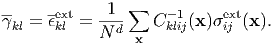
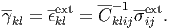
is applied to a substance, the macroscopic average γkl of the total strain is equal to the average strain ϵklext cuased by the external stress;
| (57) |
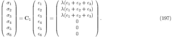
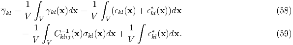
Internal strain Consider a structural phase transformation, for example, the substance with crystal lattice of cubic symmetry transforms into that of tetragonal symmetry; its eigenstrain ϵkl* is measured referring to the cubic lattice. Then, the macroscopic average of the total strain is
On the other hand, in the elastic equilibrium (i.e., ∂σik(x)∕∂xk = 0 holds) and in the absence of external force (i.e., Xi = σiknk = 0 holds, where nk is the normal vector of the surface), the sum of the internal stresses σkl(x) caused by the eigenstrain ϵkl*(x) throughout the whole substance is zero: Therefore, when the elastic constants are spatially homogeneous (i.e., Cklij(x) = Cklij), Eq. (59) is writen asExternal and internal strain The strains in both cases are summed up:
We first define a new parameter Φ(x) to prescribe which material exists at a position x; Φ(x) = 0 or Φ(x) = 1 mean the matrix or inclusion, respectively. When the difference of the elastic constants between inclusion and matrix is denoted as ΔCijkl, the elastic constants at x are written as

| (64) |
Similarly, the eigenstrain ϵkl* representing the inclusion is defined as
| (65) |
According to Eq. (70), the internal stress field is given by
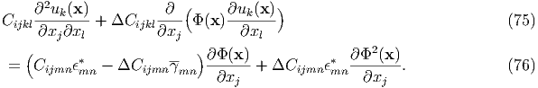
Then, the elastic-equilibrium equation is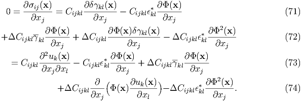
Zeroth-order approximation When the effect of ΔCijkl is neglected (i.e., ΔCijkl = 0), Eq. (76) reduces to
which is totally the same as Eq. (3). Therefore, from Eq. (8), the solution is given by
| (78) |

| (79) |
Therefore, from Eq. (55), we obtain
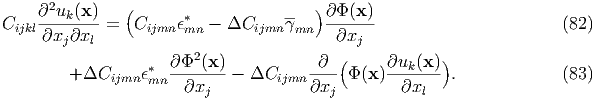
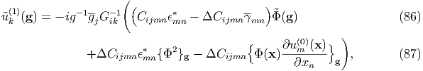
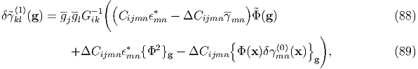
whereFirst-order approximation We write Eq. (76) as
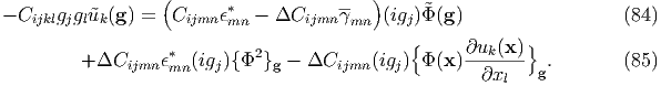
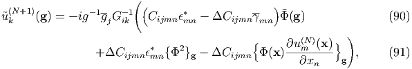
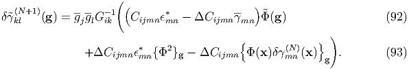
In the Fourier space, Eq. (83) is written as Since Eq. (85) is nonlinear, it cannot be soloved analytically. Thus, we obtain an approximate solution with the zeroth-order solution. The solution of zeroth-order equation uk(0) is substituted into the right hand side of Eq. (85), and a more accurate solution uk(1) is newly obtained; since C ijklgjgl = g2C ijklgjgl = g2G ik, and we obtain the (non-symmetric) total strain as where δγmn(0)(x) = ∂u m(0)(x)∕∂x n.Higher-order approximation Similarly, we obtain the higher-order solution through the iterative calculations:
and
We try to apply the discrete Fourier transformation (DFT) technique for the calculation of Eq. (80) with Eqs. (81) [0th-order solution], (89) [1st-order solution], and (93) [Higher-order solution]. For the sake of simplicity, as an example, we here treat the solution of zeroth-order approximation, i.e., Eq. (81).
| Index | xi | 0 | 1 | 2 |  | N - 1 | (N) |
| L [m] | xiΔx | 0 | Δx | 2Δx |  | (N - 1)Δx | (NΔx) |
| Index | gi | 0 | 1 | 2 |  | N - 1 | (N) |
| λ [m] |  | ∞ | NΔx |  |  |  | (Δx) |
 [1/m] [1/m] |  | 0 |  |  |  |  | ( ) ) |
In order to perform DFT, the substance is divided into Nd elements, where d denotes the dimension, and the division length is denoted as Δx [m]. Figure 3 indicates the relation between real and reciprocal spaces. With regard to physical quantities A(x) and Ã(g), the definition of DFT is given by


 ,N - 1) in the practical DFT calculation. Then, xiΔx and 2πgi∕NΔx
correspond to gi(= 2π∕λi) and xi in the conventional Fourier transformation e.g., Eq.
(11). Table 1 gives the physical quantities such as wavelength and wavenumber
corresponding to the indices, xi and gi, used in the discrete Fourier transformation.
Thus, the exponential term can be understood as
,N - 1) in the practical DFT calculation. Then, xiΔx and 2πgi∕NΔx
correspond to gi(= 2π∕λi) and xi in the conventional Fourier transformation e.g., Eq.
(11). Table 1 gives the physical quantities such as wavelength and wavenumber
corresponding to the indices, xi and gi, used in the discrete Fourier transformation.
Thus, the exponential term can be understood as

| (97) |
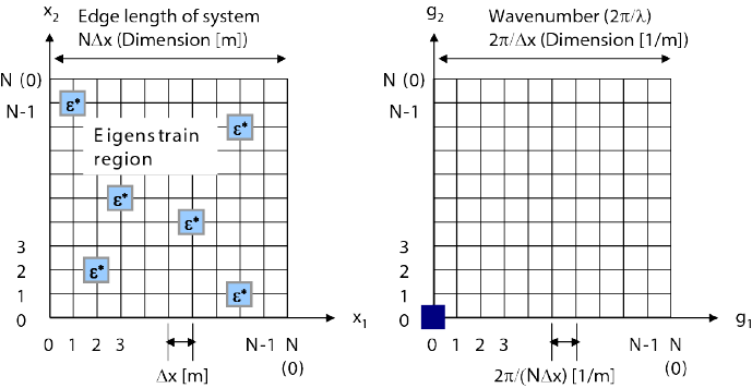
We consider the g = 0 point in Eq. (81). The DFT forms of eigenstrain  kl*(g) is given
by
kl*(g) is given
by
 kl*(0), equals the sum of ϵ
kl*(x) in the
real space (see Fig. 3).
kl*(0), equals the sum of ϵ
kl*(x) in the
real space (see Fig. 3).
In the similar way with this DFT characteristics, the following relation
should be satisfied from Eq. (54). By utilizing Eq. (100), we can avoid calculating the g = 0 point in Eq. (81). Equation (100) is the crucial key for all the calculations.
Next let us consider the constraint conditions with regard to the macroscopic-shape change. For this purpose, we rewrite Eq. (63) in the discrete form as
Furthermore, applying DFT formulae and using the characteristics of delta function Eq. (96), the total and elastic strains are expressed as and respectively, where note that ϵkl*(x) = ϵ kl*Φ(x). In the above equations, γ klδ(0) means the constraint condition, and the key is to calculate somehow the average total strain γkl.(1) Without macroscopic shape change If the substance is fixed in the rigid box, γkl = 0 should be used for the calculations.
(2) Without external stress If no external field is applied and the substance is elastically homogeneous, the average total strain is given by the spatial average of eigenstrain:

If the substance is elastically inhomogeneous, since

(3) With uniform strain Origin of the uniform strain (e.g., mechanical, electrical, magnetical sources) is not limited. Then, γkl is given as a constraint condition.
For example, when the external stress σijext is applied to the elastically homogeneous system, the external uniform strain
| (107) |
is caused. Then, when calculating Eq. (103), we use as a constraint condition
(4) With external stress Since the eigenstrain effect ϵkl*Φ(x) can be added later, we distinguish the effects of the external stress and eigenstress (eigenstrain), and here discuss the only effect of external stress.
This condition is the most general, but the most complicated in the case of the elastic inhomogeneity, which is totally different from the uniform strain condition. Because the uniform strain is usually not caused, when an external stress σklext is applied to the elastically inhomogeneous substance. The relation that necessarily holds is

| (109) |
where

Since the eigenstrain effects can be added later, this is now ignored, and then the macroscopic average γkl of the total strain equals the average strain ϵklext cuased by the external stress;
| (110) |
Usually, we do not know the detail of σijext(x), and therefore this constraint condition is somewhat complicated. If you know the effective (average) elastic constants Cklij in advance, we obtain
| (111) |
Therefore, solving this constraint problem is converted to obtaining the effective elastic constants.
The effective elastic constants Cklij obtained by the other methods are generally not self-consistent. Thus, the following iterative calculations are needed.


Remarks This method for evaluating the effective elastic constants is implicitly based on Colonnetti’s theorem, which is described next section. According to this theorem, the external stress does not interact with the elastic strain due to eigenstrain. When the substance includes the elastic inhomogeneous inclusions with an eigenstrain, the substance is in an internal-stress state, regardless of the existence of an external stress. We regard this (equilibrium) state as a standard state, and consider the case where an external stress is further applied to the equilibrium state. Colonnetti’s theorem says that the total strain energy Estr stored in the substance is given by the simple sum of the strain energy due to the eigenstrain Estrint and that due to the external stress Estrext, i.e., E str = Estrint + E strext. If the inclusion has no eigenstrain but has only different elastic constants, the strain energy is caused only by the external stress, which equals Estrext stated above. Namely, we may ignore the eigenstrain effect when considering the effective elastic costants. Once we obtain the accurate or self-consistent effective elastic constants, δγmn is to be calculated with Eq. (93) using the average total strain γmn = Cmnij-1σ ijext.
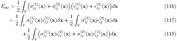
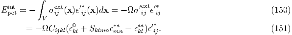
In this section, we discuss various kinds of mechanical energies. There are two types of energies to be discussed here. One is the elastic strain energy Estr, and the other is the potential energy Epot of external stress (load). The sum of these energies is called the total mechanical energy:

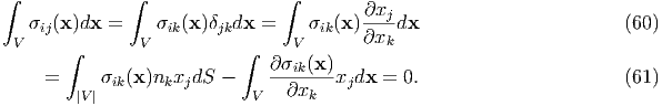
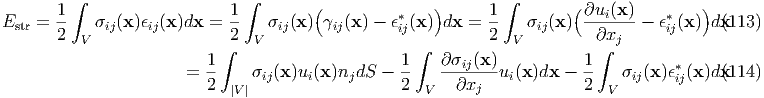
Let us consider the case where the substance has only one inclusion with eigenstrain ϵij*. The strain energy stored in the whole substance is
where σijnj = 0 on the surface |V | and ∂σij∕∂xj = 0 everywhere. Therefore,
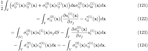
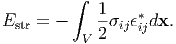
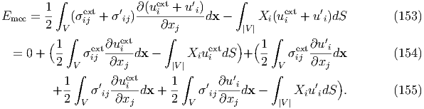
Let us consider the case where two inclusions exist in the substance, and we define the elastic interaction energy. The total strain energy due to the eigen-stresses (1) and (2) is given by


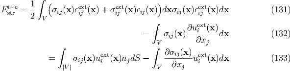
When the eigenstress/eigenstrain and the external stress/strain coexist, the elastic strain energy is expressed as
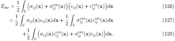

Furthermore, using the other hand, σijext(x)ϵ ij(x) = σijext(x)[γ ij(x) -ϵij(x)], in the expansion,
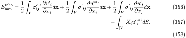
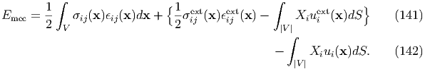
Let us consider the case where the eigenstrain and external stress coexist. Considering the potential energy due to external stress (potential energy of weight in the system consisting of spring and weight), the total mechanical energy Emec, which corresponds to the Gibbs free energy, can be defined as
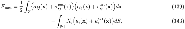
 }, is the total mechanical energy caused by the external stress,
where the former term in {
}, is the total mechanical energy caused by the external stress,
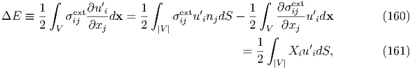
where the former term in { } means the external strain energy Estrext, and the latter
means the potential energy, Epotext, of the external load, which is expressed as
} means the external strain energy Estrext, and the latter
means the potential energy, Epotext, of the external load, which is expressed as

Remarks In the above arguments, there is no limitation or constraint on the elastic constants Cijkl, i.e., the case of elastic inhomogeneity can also be dealt with, and furthermore the shape of inclusions are not specified.
When the inclusion shape is assumed to be ellipsoidal, the calculations including volume integrals are fairly reduced, because the internal stress and strain inside the inclusion become uniform.
Elastic homogeneity From Eq. (115), the elastic strain energy is given by


Elastic inhomogeneity If an elastically inhomogeneous (C′ijkl) inclusion has an eigenstrain ϵ′kl*, using the equivalent eigenstrain ϵkl* (see section 1.4), the internal stress inside the inhomogeneous inclusion is given by


From Eq. (144), the mechanical interaction energy Epotint is
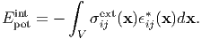
Elastic homogeneity In this case, the above equation is straightforwardly applicable, i.e.,

Elastic inhomogeneity In the case of elastically inhomogeneous (C′ijkl) inclusion, if it has no eigenstrain, Epotint is not caused. When the elastically inhomogneneous inclusion has an eigenstrain ϵ′kl*, E potint should be considered. The applied stress to the inclusion, σijext(x), is different from the originally uniform stress σ ijext(= C ijklϵkl0), i.e., σijext(x) = σ ijext + σ′ ij(x) ≡ σ′ijext. In order to know the stress inside inclusion, Type-I equivalent inclusion method, Eq. (51), is used:
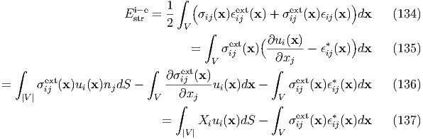
In the previous sections, the general definitions of the mechanical energies are presented. Here, we focus especially on the case where the external stress is applied to an elastically inhomogeneous substance. We are not concerned about the existence of eigenstrain regions; for the sake of simplicity, the substance has no eigenstrain regions.
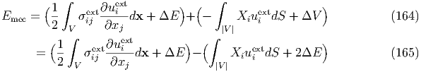
In the case where an external stress is applied to an elastically inhomogeneity, the total mechanical energy (the residual parts of Eq. (142) after removing the eigenstrain terms) is expressed as


After all, the total mechanical energy is expressed as

Application of equivalent inclusion The above argument holds regardless of the inclusion shape. We here assume an ellopsoidal-shape inclusion. Referring to Eq. (144), we apply the Type-I equivalent inclusion method to this case:


By substituting Eq. (168) into the first term of the right-hand side of Eq. (165), we can discuss macroscopic effective elastic constants. Next section presents more systematic treatment for deriving the effective elastic constants, and this strain-energy balance will be discussed in Section 4.4.
The general formulae for the effective elastic constants are to be derived based on the Eshelby’s ellipsoidal inclusion theory[1] and Mori-Tanaka’s meand-field approximation (MTMF) theory[7]. On this issue, the mathmatical treatment has been first presented by Benveniste[8]. His approach is very simple and widely applied to other relatated topics. In this section, following the procedure of Benveniste, we will present the derivation of the effective elastic constants.
Consider a composite material consisting of a matrix with the elastic constants C0 and a type of inclusion with C1, whose volume fractions are denoted by 1 - p and p, respectively. The average stress σ and average strain ϵ of the composite are approximated as σ = (1 - p)σ0 + pσ1 and ϵ = (1 - p)ϵ0 + pϵ1, where σ0 = C0ϵ0 and σ1 = C1ϵ1. The average stress σ must be equal to an external stress, because the sum of internal stresses have to be zero: ∫ V σij(x)dV = 0. Then, the average elastic constants C of the composite material can be defined as σ = Cϵ, i.e.,
![--
(1 - p)C0ϵ0 + pC1 ϵ1 = C [(1 - p)ϵ0 + p ϵ1].](MicromechanicsApplication151x.png)
| (170) |
When expressing ϵ1 = Aϵ0, the average elastic constants C of the composite can be written as
![-- -1
C = [(1 - p)C0 + pC1A ][(1 - p )I + pA ] ,](MicromechanicsApplication152x.png)
| (171) |
where I is the unit matrix. The matrix A is called the strain-concentration factor. In order to obtain the effective elastic constants C, we must find A.
The strain-concentration factor A can be derived on the basis of Eshelby’s equivalent-inclusion[1] and Mori-Tanaka’s mean-field theories[7].
We suppose first that the external stress σext is applied to an elastically uniform (elastic homogeneous) substance:

| (172) |
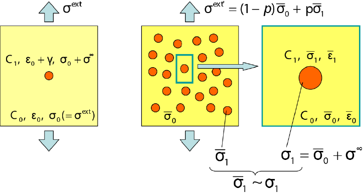
where ϵ0 denotes the uniform strain in the absence of any inclusions. Next, we consider a substance containing, in a matrix with the elastic constants C0, an infinitesimally small inclusion that has different elastic constants C1 but has no intrinsic eigenstrain such as a lattice misfit, and consider the case where an external stress σext is applied to such an elastically inhomogeneous substance. Then, the internal stress σ1 inside the inclusion is given by

| (173) |
where σ∞ and γ represent the disturbances of internal stress and strain. which are caused by the elastic inhomogeneity under an applied stress. Such a situation is depicted in Fig. 4. When the inclusion is ellipsoidal, according to Eshelby’s concept, Eq. (173) can be expressed using the eigenstrain ϵ* of “the equivalent inclusion” as

| (174) |
where the extra strain γ is given by γ = Sϵ* with S the Eshelby tensor. Hence, σ∞ can be expressed as
| (175) |
If σ∞ is expressed without using the Eshelby tensor S,

| (176) |
When ϵ0 = 0 or σext = 0, the stress disturbance is not caused i.e., σ∞ = 0 and therefore γ = 0. When ϵ0≠0 or σext≠0, σ∞≠0 and therefore γ = 0 because of S≠I in Eq. (175). Thus, σ∞ and γ are functions of σext or ϵ 0.
We deal with a composite material with a large number of inclusions. Under an external stress σext′(≠σext), the average stresses and strains of matrix and inclusion are denoted as σ0,ϵ0 and σ1,ϵ1, respectively. (Then, σext′ = (1 - p)C 0ϵ0 + pC1ϵ1 holds.) The differences between σ1 and σ0 and between ϵ1 and ϵ0 are denoted by σ′ and γ′, i.e., σ1 = σ0 + σ′ and ϵ1 = ϵ0 + γ′.
On the other hand, Mori-Tanaka’s mean-field (MTMF) theory[7] allows us to express the average internal stress of inclusions as
| (177) |
Equation (177) can be understood as follows; see Fig. 4. We suppose that new one inclusion is further added into the matrix of the composite with numerous inclusions. As stated in the previous paragraph, in the case of single inclusion, the stress disturbance due to the inclusion embedded in a matrix with the external uniform strain ϵ0 (caused by σext) is given by σ∞. Since the new inclusion is to be embedded into the arleadly stressed (or strained) matrix with σ0 (or ϵ0), the internal stress of new inclusion is approximately given by sum of σ∞ and σ 0, i.e., σ1 ≈σ0 + σ∞. Moreover, as far as σ0(x) is not so much deviated from σ0, we may regard that the internal stress σ1 of the newly added inclusion is virtually equal to the average internal stress σ1 of inclusions in the pre-added original composite, i.e., σ1 ≈ σ1. Therefore we obtain σ1 ≈σ0 + σ∞. It should be noted here that we have to use σ∞ in the situation that ϵ 0 equals ϵ0. After all, we find that σ′ = σ∞(ϵ 0) and γ′ = γ(ϵ0).
Then, by using Eq. (175) based on the equivalent inclusion concept, we can write Eq. (177) as

| (178) |
Here, expressing A as
| (179) |
and substituting Eq. (179) into eq. (178), we obtain
![-1 - 1
A = [SC 0 (C1 - C0 ) + I] .](MicromechanicsApplication161x.png)
| (180) |
Essentially, the similar treatment is applicable to this case. The species of the component phases are denoted i. Then, the effective elastic constants can be expressed as
| (181) |
where ∑ ipi = 1. The average strain of i phase is denoted as ϵi, and we write ϵi in the similar way to Eq. (179) as
| (182) |
where Ai represents the strain-concentration factor of i phase, which is given (in the regime of Mori-Tanaka’s mean-field theory) by
![Ai = [SC -0 1(Ci - C0) + I]-1.](MicromechanicsApplication165x.png)
| (183) |
Note that Eq. (183) satisfies A0 = I.
We here consider the case of porous material; pore can be regarded as inclusion with C1 = 0. Here, the slightly different way of derivation of A is presented. First, let us consider the case where the single pore exists in an infinite matrix. Since σ1 = C1ϵ1 = 0 holds in Eq. (174), the following relation

| (184) |
must hold. Namely, according to the magnitude of an external stress σext, γ is determined to be

| (185) |
so as to guarantee that σ1 = 0. As mentioned abobe, one can find that γ is a function of σext or ϵ 0.
Next a porous composite is considered. Since under an external stress σext′,
| (186) |
holds, substituting C1 = 0 into above equation, we obtain σext′ = (1 - p)C 0ϵ0. In order to refer to the case of an infinitesimal single inclusion, we suppose the case where the average strain ϵ0 of the matrix is equal to ϵ0;
| (187) |
i.e., σext′ = (1 - p)σext in the case of ϵ 0 = ϵ0. Referring to ϵ0 + γ = Aϵ0 [Eq. (179)], we obtain
| (188) |
or from Eqs. (179), (185) and ϵ0 = ϵ0, we directly obtain
| (189) |
Eliminating σext′ or ϵ 0 in both hand sides, after all we obtain

| (190) |
which is consistent with Eq. (180) in the case of C1 = 0.
Other derivation of A From the equations,
and
we obtain

| (191) |
For porous materials, since σ1 = 0,

| (192) |
Hence,

| (193) |
and from this equation we obtain
| (194) |
Therefore, from ϵ0 + γ = Aϵ0 [Eq. (179)],
| (195) |
which is the same as Eq. (188).
When the shear modulus of liquid is assumed to be zero, using the Lam constant (λ
and μ = 0), the elastic constants of liquid is expressed as
constant (λ
and μ = 0), the elastic constants of liquid is expressed as
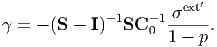
Rigid body can be regarded as inclusion with C1-1 → 0; even when an external stress is applied to the rigid body, the external strain is not caused, i.e.,
| (198) |
and therefore γ = -ϵ0. Since C1 →∞ and ϵ1 = 0, σ1 = C1ϵ1 formally has an indeterminate form, and σ1 represents the virtual stress applied to the rigid-body inclusions. This virtual stress is, of course, not a real stress of rigid body, but is the quantity that guarantees the average stress of matrix satisfies (1 -p)σ0 = σext′-pσ 1 in the case of composite.
First, we consider the case where a single rigid body exists in an infinite matrix. Therefore, Eq. (174) can be written as

| (199) |
must hold, and therefore
| (200) |
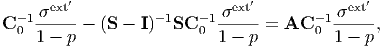
Next a composite with numerous rigid-body inclusions is considered. In this case, it is convenient to consider the stress-concentration factor, not the strain-concentration factor A, because A ≡ 0 from Eq. (198). The average elastic compliances C-1 of the composite material can be generally defined as ϵ = C-1σ, i.e.,
![(1 - p)C- 1σ0 + pC -1σ1 = C--1[(1 - p )σ0 + pσ1].
0 1](MicromechanicsApplication186x.png)
| (201) |
When expressing σ1 = Bσ0, the average elastic compliances C-1 of the composite can be written as
where the matrix B is called the stress-concentration factor. From Eq. (177) and σ1 = Bσ0, we obtain
| (203) |
Comparing with Eq. (200) obtained for a rigid body, we find
| (204) |
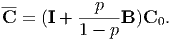
where B = S-1 when C 0S-1 = S-1C 0 holds. Since we can regard that C1-1 = 0 for rigid bodies, from Eq. (202), the average elastic constants for composite with rigid-body inclusions are expressed as
| (205) |
Thus, when p → 1, the effective elastic constants are diverged. However, since p∕(1 - p) ~ O(1) when p < 0.99, this divergence takes place steeply in the vicinity of p = 1.
In the previous arguments, we considered the effective elastic constants on the basis of Hooke’s law, (1 - p)σ0 + pσ1 = C[(1 - p)ϵ0 + pϵ1], with the average stress and strain. Here we consider this matter in terms of the external strain energy caused by an external stress σijext.
When the substance is uniform, the external strain energy is given by


In the matrix form, we can rewrite Eq. (212) as
where σext(T) means the transposed matrix of σext. Eliminating (1∕2)σext(T), By substituting the following equations,
into the right-hand side of Eq. (214), and taking notice of ϵ1 = ϵ0 + γ and (1 - p)ϵ0 + pϵ1 = ϵ, we obtain
![- 1 ext *(∞ ) -1 - - - 1 -1
C 0 σ + pϵ = C 0 [(1 - p)C0 ϵ0 + pC0 (ϵ0 + γ - S γ )] + pS γ (215 )
(216 )
- - -1 - 1 - -
= (1 - p)ϵ0 + p(ϵ0 + γ - S γ) + pS γ = (1 - p)ϵ0 + p(ϵ0 + γ) (217 )
(218 )
= (1 - p)ϵ + pϵ = ϵ. (219 )
0 1](MicromechanicsApplication202x.png)
![-- -- -- - -
(1 - p)σ0 + pσ1 = C [(1 - p)ϵ0 + p ϵ1],](MicromechanicsApplication203x.png)
In general, the MTMF theory does not yield accurate elastic constants for large p, because Eq. (212) does not consider the elastic interaction between inclusions. One of the essential reasons of this problem is that the important conclusion of Mori-Tanaka’s theory, = + σ∞, does not hold when the fraction of inclusions is fairly large, where and are the average stress fields of the matrix and inclusions, and σ∞ denotes the stress disturbance caused by a single inclusion formed in an infinite matrix. This is because the elastic-interaction effect between inclusions cannot be neglected any longer. This means that we should avoid deriving directly the elastic constants for a composite with a high inclusion fraction from those of the non-inclusion material with the conventional MTMF theory. With this in mind, we here consider the evaluation method of effective elastic constants for large p.[9]
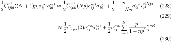
Equation (212) is rewritten as
where the superscript (0) means p = 0, Cijkl-1(0) and ϵ ij*(0) represent C ijkl-1 (the elastic compliance of matrix) and ϵij*(∞) in the previous section. Namely, ϵ ij*(0) is the equivalent eigenstrain that is prepared referring to the substance without any inclusions. Equation (220) is fairly accurate when p ≪ 1. We consider the case where the fraction of inclusion is further increased, for example, to 2p. According to Eq. (220), the effective elastic constants for 2p is given by However, there is no longer guarantee that Eq. (221) is accurate, because we cannot judge whether 2p ≪ 1 or not (even if p ≪ 1). If we believe that Cijkl-1(p) obtained for p ≪ 1 from Eq. (220) is accurate, we had better use the following equation, instead of Eq. (221): where ϵij*(p) is the equivalent eigenstrain that is prepared referring to the homogeneous substance with the elastic constants Cijkl-1(p), in which influences of the inclusions are renormalized. The elastic constants Cijkl-1(2p) obtained from Eq. (222) are more reliable than those obtained from Eq. (221), because the condition of p ≪ 1 is still used in the equation. Thus, in the case of (N + 1)p, we can write successively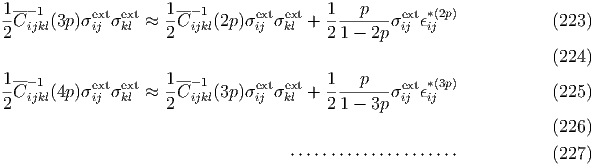
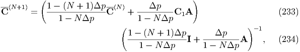
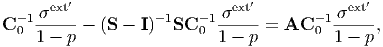
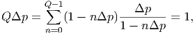
As seen in the previous section, the strain-energy balance equation (209) is totally equivalent to Eq. (171) with Eq. (180) derived on the basis of Hooke’s law σext = Cϵ. Therefore, Eq. (171) is still used in the EMF treatment, but is applied only in the low fraction range. Namely, C0 in Eq. (171) is sequentially superseded by C (effective elastic constants) for a lower fraction obtained by a previous calculation step, and then the effective elastic constants of a renewed composite with a slightly higher fraction are to be calculated. When the increment of fraction with regard to the original non-porous material is given by Δp, the division number Q of the entire fraction range (0 ≤ p ≤ 1) is Q = 1∕Δp (Δp should be chosen in order for Q to be integer). Then, the following relation,
| (231) |
holds, where 1 - nΔp means the fraction of the previous (pre-renewed) porous sample and Δp∕(1 - nΔp) represents the virtual fraction measured referring to the previous porous sample that is regarded as a matrix. Therefore, the fraction p of a renewed porous sample is expressed as

| (232) |
Based on the above concept, Eq. (171) is modified as a following formula:
where C(N+1) and C(N) are the effective elastic constants of the renewed and previous porous samples, respectively. It should be noted that the strain concentration factor A and the Eshelby tensor S have to be calculated using C(N). Furthermore, C(N) is not always isotropic even if the initial matrix is elastically isotropic. For an anisotropic medium one has to calculate the Eshelby tensor using Eqs. (45)-(47).
[1] Eshelby, J.D., Proc. Roy. Soc. London, A241 (1957), 376.
[2] Mura, T., Micromechanics of Defects in Solids, Second, Revised, Edition (Martinus Nijhoff Pul., The Hegue, 1987).
[3] Mura, T. and Cheng, PC., J. Appl. Mech., 44 (1977), 591.
[4] Kinoshita N. and Mura T., Phys. Status Solidi, A5 (1971), 759.
[5] Khachaturyan AG, Theory of Structural Transformation in Solids (Wiley, New York, 1983).
[6] Hu SY. and Chen LQ., Acta Mater. 2001, 49 1879.
[7] Mori, T. and Tanaka, K., Acta Metal., 21 (1973), 573.
[8] Benveniste, Y., Mech. Mater., 6 (1987), 147.
[9] Tane, M. and Ichitsubo, T., Appl. Phys. Lett. 85 (2004), 197.


![[ ]
γ- + δγ (x) = -1- ∑ γ- δ(g) + δ˜γ (g ) exp(i2π-g ⋅ x ) (102 )
kl kl N d g kl kl N](MicromechanicsApplication99x.png)


![--- 1
C = [(1 - p)C -01+ pC -11B ][(1 - p)I + pB ]-1, (202 )](MicromechanicsApplication187x.png)